Updated: 6 March 2011

Advisor: Hiro Yamamoto
LIGO, Caltech

^∗(Also an Research Experiences for Undergraduates Program)

Publications and Presentations

1. "Gravitational-wave Signal Simulation for LIGO," 2002, 16th National Conference on Undergraduate Research, University of Wisconsin−Whitewater (presentation PDF and proceeding below)
2. Cooksey and Yamamoto, "Gravitational-wave Signal Simulation for LIGO," 2002, LIGO Document Control Center, (PDF; also NCUR proceeding)

ABSTRACT

The Laser Interferometer Gravitational-wave Observatory (LIGO) has been constructed to directly measure the distortion of spacetime due to an impinging gravitational-wave (GW). LIGO's biggest challenge is that the size of the signal is tremendously weak, and there are various kinds of noises that need to be suppressed to make the tiny signal visible. In order to assist in tackling this issue, an end-to-end time domain simulation program for LIGO (E2E) has been developed to simulate the detector response to a signal caused by a GW and to various kinds of noises under a realistic operational condition. The latter can be simulated already in the existing E2E. In order to simulate the response of LIGO to the signal of GW sources, a new software program has been developed for E2E. In this paper, the details of this software are discussed. This program calculates the time- series variation of the strain for coalescing compact binaries and spin-down supernovae. The program is flexible in choice of source and detector location and orientation and generates signals with proper correlations due to spatial separations and detector orientations. The program also visualizes the time-series of the result for one interferometer's detection or for multiple, correlated detections.

1. Introduction

The Theory of General Relativity predicts the existence of GW, oscillations in the fabric of spacetime due to the acceleration or non- axisymmetric motions of massive objects. Such objects radiate GW with different patterns depending on the motion of the source. GW propagates at the speed of light [1] and theoretically have two orthogonal polarizations, called in this paper, plus and cross [2]. The net affect of these polarizations is a plane that distorts spacetime, causing one direction to stretch as the perpendicular direction contracts. The strain is the fractional change of length along a polarization axis.

(1)

where L0 is a length of a distance when there is no GW, and L is the same length when there is space distortion. A physical quantity which is easier to measure is the difference of two distances perpendicular each other.

(1')

where L_x and L_y are measured distances along the x- and y-direction, respectively. When the x-axis is chosen to be along a polarization axis, these two quantities are the same.

In addition, GW can pass through most matter without significant change, and the strain weakens as the inverse of the distance [3]. In this manner, GW not only offer a new way to observe the cosmos but they also carry their information farther and in a more pristine package.

LIGO has three interferometers at two sites: one 4-km and one 2-km interferometer at Hanford, WA, and one 4-km interferometer at Livingston, LA. These interferometers consist of six mirrors suspended in vacuum chambers, forming Michelson interferometers with long Fabrey-Perot arms. They are designed to detect changes on the order of 10^-18 to 10^{- 22} m. Currently, both sites are undergoing engineering work and being fine-tuned to increase their sensitivity [4].

E2E simulates the LIGO detector system, factoring into account laser fields, resonant optical cavities, mechanical systems, control system, et cetera, and it tries to simulate the LIGO detector as realistically as possible. E2E has major noise sources already programmed, such as seismic, thermal and shot noises. Other secondary noise sources, like laser frequency and electronic noises, are added when they become a large noise factor.

The simulated time series of data, which contains known amounts of noises and the signal, can be used to develop the data analysis algorithm. The latter software needs to have a high efficiency of detecting signals with very low misidentification rate of the noise as a signal. E2E did not have a code to generate strains caused by GW sources. A new program has been written to generate the strain of major GW sources, which can be used by E2E to simulate the data with mixture of noises and signals. The new program generates a data file, which contains data of strains of each arm, and E2E reads this file to generate data caused by the GW source. In this paper, the details of this program are discussed.

The two major signal sources that the simulation program generates are discussed in section 2. Section 3 is devoted to the details of the formulation used in the program. The program structure and instructions for use are given in section 4. Section 5 is a summary of this program and possible future uses, improvements, and results.

2. Signal Sources

The program simulates two GW sources: compact binaries and supernovae. The general formula for the GW strain is composed of geometric coefficients and polarization strains [4]:

(2).

θ and φ are polar coordinate angles that define the location of the source in spherical polar coordinates in the earth coordinate system, and ψ is the angle of rotation of the polarization x-axis from the constant φ plane (Fig. 1) [5]. The polarization strains h₊ and h_× are calculated by the dynamics of the GW source, and depend on time and source location in the sky. The actual strain measured depends on the relative orientation of the detector to the signal direction and the polarization axis. The coefficients F₊ and F_× account for this geometrical effect.

Figure 1: Source location and orientation in the earth coordinate. Light gray lines indicate projections toward the background.

Compact binaries are inspiraling and coalescing pairs of neutron stars and/or black holes. These GW sources are the most understood and have the best models. Gravitational radiation carries the energy away, causing the pair to coalesce. The rapid rotation of the system propagates stronger waves. The strain increases in amplitude and frequency as the binaries merge, the so-called "chirp" signal [4].

There are several ways by which supernovae can generate GW. The new neutron star could "be convectively unstable and 'boil' vigorously" [4]. A rotating star in pre-supernovae stage might collapse and bulge perpendicular to the axis of rotation. If this core has small angular momentum, it would most likely be axisymmetric and emit low-amplitude GW. On the other hand, if the angular momentum is large, the core may be non-axisymmetric and break apart, producing strong GW. When the core becomes hung-up just before its final neutron star phase, GW are emitted at a high frequency, decreasing to low frequency. This spin-down supernova case is simulated in the simulation program.

The explicit formula of strains for these signals can be found in references [4] and [6]. The formulas used in this program are slightly different from those in these references due to needed updates. The differences are summarized in section 4.

3. Formulation

The program uses the polarization strains and the geometry of the source and detector to calculate strains for the x- and y-arms:

	(3) and
	(4).

For E2E, the arm strains, defined as equation (1), are used to simulate the GW source. E2E simulates LIGO by moving the test masses, effectively changing the arm lengths, in response to an external source (e.g. background noise). Strictly speaking, the effect of the GW source is slightly different from the physical displacement of test masses but this is a very good approximation.

As is shown in equation (2), the program needs to account for the location and orientation of the source and detector. Then E2E uses the arm strains to move the test masses the correct amount in the respective arms. By simulating the effect for each arm, realistic as-built interferometers with imperfections can be calculated in E2E simulation. For example, E2E can simulate the case where the arms are not locked to precisely the same length.

The F coefficients are due to the orientation of the source and detector. The polarization strains characterize the change in the detector were it perfectly aligned with the plus and cross polarizations, respectively. The coefficients are a matrix transformation from the detector coordinate system to the polarization coordinate system. The subscripts reflect which arm has been transformed to which polarization. In the detector coordinate system:

	(5).

These coordinates are transformed to the earth coordinate system using the arm angle (Fig. 3) and the detector location in latitude and longitude (Fig. 2). The new coordinates of each arm are next transformed to each polarization system through the polar coordinates and the polarization rotation (Fig. 1). This process yields the full F coefficients.

Figure 2: Detector location as defined by latitude and longitude.

Figure 3: Detector orientation by the arm angle as shown above.

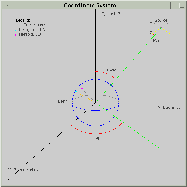
The geometry of the detector and source has an important impact on GW detection. The strain is on the order of 10^-18 to 10^{- 22}, and it is difficult to discern a true detection from unknown background noises. Therefore, LIGO depends on correlated detections at its two sites. The location of the detectors with respect to the source determines which site will be affected first (Fig. 4).

Figure 4: Time delay as a function of opening angle α, radius of the earth R_earth, and speed of light c

(6)

In addition, the detector orientation affects the amplitude of the strain in the waveform, the graph of the time-series variation of the strain. The waveform has characteristic shape for each type of source and, in general, offers an intuitive visualization of the variation of the strain. For the simulation program, the total strain for a GW source is:

(7).

Therefore, a true GW detection can best be verified by three aspects of the waveforms: correct time delays due to spatial separation, characteristic shape for the source type, and appropriate amplitude due to detector orientation.

4. Design and Instructions

The signal simulation program is an interactive JAVA program that can calculate the time-series of the strain for a coalescing compact binary or spin-down supernova and visualize the waveform for single or multiple detections. The interface displays simple line-by-line prompts that describe the requested quantity, its allowable range, and offer default values. Every entered quantity is checked so that it falls within the specified range. The default values are for convenience when no value is preferable or guidance if there is a recommended value.

The program is menu-driven with four choices: (1) simulate compact binary; (2) simulate supernova; (3) graph waveform; and (4) overplot multiple waveforms. For the simulation options, the first prompt is for a filename with no extension because this name will be used for two files: a data (*.dat) file and an information (*.info) file. The former must be strictly columns of numbers, and the information file contains the parameters the user entered and other such pertinent quantities.

Next, the user is prompted for the detector and source location and orientation. There are six GW interferometers already programmed with their pertinent global coordinates and orientation (Table 1). In addition the user may opt to enter the values for a new detector. The latitude and longitude do not have default values but are constrained to be positive values in the appropriate ranges. The matrix transformation from detector coordinates to earth's depends on a specific definition of the x-arm angle; the x-arm must align with due south and the y-arm with due east after transformation. 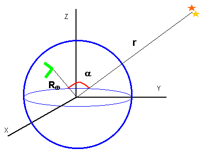In order to constrain the user to this definition, he merely enters the quadrant of the x-arm (Fig. 3) and the angle from a specified axis. Then the program adds or subtracts 90° as necessary depending on the quadrant. The source location and orientation are simply entered via angles with respect to the earth coordinate system (Fig. 1).

All angles given in degrees and defined by Fig. 2 and Fig. 3 [7].

Now the program prompts become more specialized to the source being simulated. The user is required to enter several quantities pertinent for the calculations such as mass(es), inclination angle, et cetera. The compact binary equations are second post-Newtonian equations and are used as given in reference [4]. The supernova equations were discovered to be outdated. GRASP documents a supernova formula but uses a different one in the code. First, all units must be converted to the cgs system unless otherwise noted in the documentation. Solar masses must be converted to geometric units: one solar mass equals about 1.477x10⁵ cm. Second, equation (14.1.3) of GRASP is as follows:

(8).

The change is that A1 replaces A, equation (14.1.2):

(9).

For both references, the geometric coefficients F in equation (2) are different because LIGO's simulation program accounts for detector location and orientation as well as the source's. These are the only correction made to the equations in references [4] and [6].

Two important values that are common to both the simulation of a compact binary and a supernova are the time increment and the frequency range. The value of the time increment will effectively reflect the sampling rate of the detector.

The frequency range enables the simulation to truncate the data to that which falls in the detector's bandwidth. The program simulates in the time domain and calculates the time range via the frequency range. In the compact binary case, the program iteratively searches for the time range, which corresponds to the specified frequency range. Since in the supernova simulation, the frequency decreases, the program simply ends its calculation once the frequency drops below the specified minimum.

Once the necessary values are entered, the program prints those values to the information file. Then it calculates the time-series variation of the strain and prints three columns to the data file: correlated time, x-arm strain and y-arm strain. The correlated time is the time that was used to calculate the strains plus the time delay due to the geometry of the detector and source. The detection is correlated between the detector and the center of the earth (Fig. 4). The simulations begin time at zero, and the time delay can be a negative quantity. Therefore, the data file can have negative times. The start time may not be the time delay because the program truncates the simulation based on the frequency range. The user knows the time delay and time range from the information file.

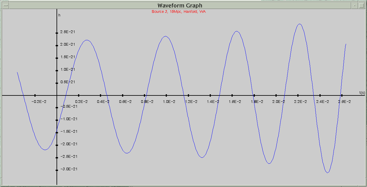
For source simulations, the program rereads the data file and displays the waveform (Fig. 5).

Figure 5: Compact binary waveform for 2 10 M_sun objects at 15 Mpc detected at Hanford, WA, in frequency range of 100 Hz to 10 kHz.

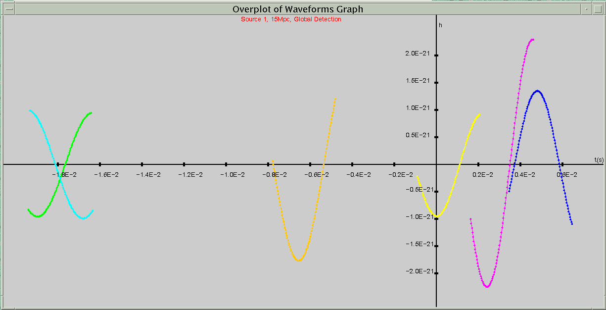
Automatically correlating the time for a simulation in the data files is most important for comparison waveform graphs (Fig. 6). Overplotted waveforms, option 4, allow the user to instantly see the time delays between detections at different sites and amplitude differences due to detector orientations.

Figure 6: Compact binary comparison waveform graph for 5 and 4 M_sun objects at 15 Mpc, in frequency range 100 Hz to 10 kHz, detected at: 40-m, California Institute of Technology, Pasadena, CA (blue); Livingston, LA (pink); Hanford, WA (yellow); GEO, Hanford, GER (green); TAMA, Tokyo, JPN (orange); and VIRGO, Pisa, ITA (blue).

The signal simulation program is a new E2E addition that can be improved. First, the user interface could be a single GUI to accept and check all values at once for one simulation. Then the program could display a customized graphic of the source and detector location and orientation. All GUIs, including the actual waveform graphs, could be improved by using more sophisticated JAVA classes (e.g. swing). Second, the graphing could allow more user-input, such as location of labels, colors, and tick sizes. Third, the user could be allowed to choose what data is printed to the data file. For example, the time could be printed with or without time-delay. The content of the columns could be user-selected (e.g. the frequency variation of strain, time-variation of the total strain or polarization strains). Fourth, the simulation program could use the data to generate noise, such as a "chirp" signal [4]. Lastly, the program could simulate more sources. This merely requires a class to calculate h₊ and h_× and addition to the main in the same format as for compact binary and supernova. As mentioned in section 2, there are other types of supernovae to simulate. Two other main sources of GW are pulsars and stochastic background noise, which can be simulated [4].

5. Conclusions

The signal simulation program calculates the time-series variation of the strain for two GW sources and visualizes the waveforms. The program calculates the strains of a GW signal, taking into account the orientation of the detector arms and the delay of the signal arriving at different locations. The output of this program can be used by E2E to simulate the LIGO detector and to generate data series with GW signals and with various noises.

The program and its documentations are available on a LIGO website [7].

6. Acknowledgements

I would like to thank Dr. Yamamoto for his support and guidance. I thank the CIT SURF program and LIGO/ NSF REU for the opportunity to do research. LIGO is supported by the National Science Foundation under the cooperative agreement PHY-9210038.

7. Reference

1. "Large Scale Measurements" Science, Vol. 256 (17 Apr. 1992) pp. 281-412.
2. B. C. Barish, R. Weiss, "LIGO and the Detection of Gravitational Waves" Physics Today (Oct. 1999).
3. Pavilion of Science and Industry, NCSA Science for the Millennium, http://archive.ncsa.uiuc.edu/Cyberia/Expo/science-pavilion.html.
4. J. K. Blackburn, "The Laser Interferometer Gravitational Wave Observatory Project" (Laser Interferometer Gravitational-Wave Observatory, Mar. 1996).
5. P. R. Saulson, Fundamentals of Interferomic Gravitational Wave Detectors (World Scientific, 1994).
6. B. Allen, GRASP: a Data Analysis Package for Gravitational Wave Detection (University of Wisconsin – Milwaukee, May 2000) http://www.lsc-group.phys.uwm.edu/~ballen/grasp-distribution/.
7. K. Cooksey, TheoryWaveform, http://www.ligo.caltech.edu/~e2e/signal/kcooksey.